Material back orders are a common problem in supply chain management system. It happens when a demanded product has gone out of stock and the retailer/manufacturer fails to fulfill the order. This article is based on a machine learning case study which predicts the probability of a given product to go on back order, using ensemble ML algorithm. The ML problem was appeared in the Kaggle Challenge “Predict Product Backorders”.
What are Back-orders?
Back-orders are those orders that are placed in the unavailability of sufficient stock. But how can someone place an order if there is no stock left for supply..?
These are placed with a promise by the supplier that the product would be delivered within a short period of time. Back orders usually happen with premium or luxury products which are high in demand, and for which customers are willing to wait (eg: latest model of iphone). However, back-orders ensure the customer that the product will be made available within a short period,even if it is currently out-of-stock.
Business Problem:
Although back orders seem to reflect the increased demand of a product, on the other side, it could be the result of poor supply chain management system. Back orders can be worse if not handled properly. Increased number of back orders could result in
● Unnecessary charges for labor ,transportation and storage
● Loss of customers by making them wait for longer
● Loss of sales
● Reduced gross profit
● Reduced market share
● Affects goodwill of the business
Back orders affect the efficiency of the business and may lead to huge loss. Forecasting the probability of stock-outs and back orders prior to its occurrence can help the situation.
This case study tries to minimize the effects by predicting the products which are likely to go on a back order weeks before its occurrence, so that businesses can take necessary actions at an earlier point of time, thus improving overall efficiency.
Machine Learning Problem:
Machine learning models that are learned from past inventory data can be used to identify the materials that are at the risk of back order before the event occurs. The model identifies whether a product will go on back order or not. So this problem can be mapped into a binary classification problem which classifies the products into:
● products that tend to go on back order as positive class(‘went_on_backorder’, labelled 1)
● Products that are less likely to go on back order as negative class(labelled 0)
Business Constraints:
● Feature Interpretability is important
● No strict latency constraints
Evaluation metrics:
AUC : ROC Curve is plotted between false positive rates and true positive rates obtained by the model predictions at various thresholds. Area Under the ROC curve can be interpreted as the probability that a given classifier ranks a random positive example above a random negative example. An ideal classifier gives an AUC value of 1 whereas a random classifier gives an AUC of 0.5. AUC less than 0.5 denotes a classifier worse than random classifier. Here AUC is chosen as the primary metric
2.Precision,Recall and F1 Score:
● Precision indicates how confident the model in its prediction and
● Recall indicates how well the model is, in predicting all positive points correctly.
Here we are interested in detecting as much as points that tend to go on back order, ie., the positive class. Recalling all the positive points correctly is important here because the cost of miss classification is higher for not detecting a back order(low recall) than labeling a product that won’t go back order as a product that would go back order ( low precision)( However,this could vary with the domain). But we can’t compromise too much on precision. So we also compute F1 score ,which is the harmonic mean of precision and recall.
The Data set
The data set was appeared in Kaggle’s competition ‘ Predict Product Backorders’ , and is now available in this github profile. It contains ~1.9 million observations ,22 features and the target variable. The features are:
● sku: unique product id
● national_inv- Current inventory level of components.
● lead_time -Transit time between placing the order at manufacturer and
receiving at retailer.
● in_transit_qty — Quantity in transit
● forecast_x_month — Forecast sales for the net 3, 6, 9 months
● sales_x_month — Sales quantity for the prior 1, 3, 6, 9 months
● min_bank — Minimum recommended amount in stock ( safety stock)
● potential_issue — Indicator variable noting potential issue with item
● pieces_past_due — Parts overdue from source
● perf_x_months_avg — Source performance in the last 6 and 12 months
● local_bo_qty — Amount of stock orders overdue
● X17-X22 — General Risk Flags
●
went_on_back_order — Whether the product went on back order, Target
Variable
Exploratory Data Analysis (EDA)
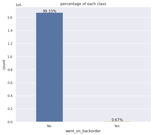
1. ‘went_on_back order’:
The target variable takes two values:‘Yes’ & 'No’(1 & 0) which interpret whether the product has gone on back order or not.
In the data set , more than 99% of the observations belong to class 0 .ie., majority of products did not go on back order. Only a small percentage of products did go on back order. Clearly, the data set is highly imbalanced with percentage of minority class less than 1.
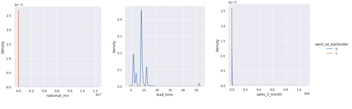
2. Continuous features
national_inv,lead_time, in_transit_qty ,forecast_x_month , sales_x_month, min_bank ,pieces_past_due,perf_x_month_avg are the continuous features in the dataset.plotting their distribution:
From the plot it is clear that most of the features are highly skewed to the right. There are large no. of small values and very few no. of large values for these variables.
These large values need not necessarily be outliers as this is sales and inventory data and there can be wide range of sales,prices, quantities depending on size of business,product variety available etc. But extreme high values might be anomalous.
There are large negative values in the inventory feature(may be because of errors in data) and missing values in perf_x_month_avg and lead_time.
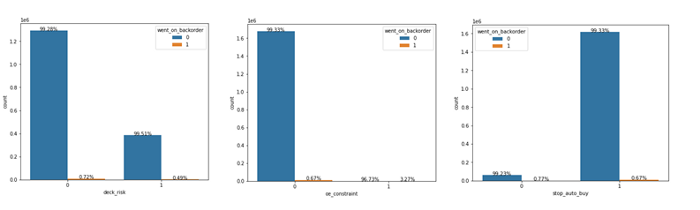
3. Discrete Features
The distribution of some of the discrete features is as shown below:
Discrete features include stop_auto_buy, ppap_risk, oe_constraint, deck_risk, potential_issue etc. More than 99% of the observations have value 0 for these flags except for stop_auto_buy flag. For this flag, majority of points have value 1. However distribution of target is similar across both flag values.
Feature Correlations
Feature correlations are used to determine interdependence between features. Plotting the correlations:
From the plot, it is clear that
● Features like in_transit_qty, forecast_x_month, sales_x_month and min_bank are highly correlated to each other.
● Inventory- sales ,min_bank features,All the three forecast features,sales features are positively correlated with each other.
● stop_auto_buy -lead time and deck_risk -perf_X_month_avg shows negative correlation.
● No feature shows high correlation with target.
Training Methodology:
Train-Test split:
For training and testing, the whole dataset is splitted into train and test data in the ratio 80:20 with stratified sampling as there is huge imbalance. This will split the data set with similar distribution of target in both parts.
This is done before any other processing , and the pre-processing steps were applied on train and test data separately to prevent any kind of data leakage.
Data-pre processing:
from sklearn.model_selection import train_test_split
data,test=train_test_split(data,test_size=0.2,stratify=data['went_on_backorder'])
From the EDA performed, It is clear that
● There are missing values
● The features are highly skewed.
● Some features are highly correlated
→ The missing values are imputed with the median.
→ Some data transformations like Log-transform and square transform are applied to reduce the skewness. ‘ ‘
→ The features ‘forecast_3_month’,‘forecast_3_month’,‘forecast_3_month’ are highly correlated each other.
Similarly, ‘sales_1_month’ , ‘sales_3_month’, ‘sales_1_month’, ‘sales_1_month’ are also correlated and shows a linear relationship. Only ‘forecast_3_month’ and ‘sales_3_month’ are kept and discarded the rest, as they do not add any value to the model.
→ Also, ‘sku’ is unique to each row and adds no value to the classification. So this featue is to be discarded.
#Missing value imputation
med=np.median(data[data['lead_time'].notnull()]['lead_time'])data['lead_time'].fillna(med,inplace=True)
#Log-transform
data['in_transit_qty']= data['in_transit_qty'].apply(lambda x: np.log(abs(x)+1)*np.sign(x))
#square transform
data['forecast_3_month']=data['forecast_3_month'].apply(lambda x: x**2)
Feature Scaling
Some machine learning models will perform better when the data is scaled. Normalization and standardization are two common techniques for this. Normalization scales values to the range (0–1). A value is normalized as follows:
#normalization
y = (x — min) / (max — min)
Standardization makes the values to be zero-centered with a unit standard deviation. This means that after standardization the mean will be zero and standard deviation will be one.
Here’s the formula for standardization:
#standardization
y= x - mean(x) / std_deviation
In the dataset all the continuous features were standardized using sklearn standard_scaler.
Feature Engineering
Feature engineering is the process of creating new features from existing raw data,using domain knowledge. In this problem I engineered few features :
1. Reorder Point (ROP)
The point of inventory level at which you need to order a product or parts before you start using your safety stock.
2. usable_stock:
This feature indicates that how many stock is left to reach the reorder point.
data[‘usable_stock’]=data[‘national_inv’]-data[‘reorder_point’]
Reorder Point = Safety Stock + Average Daily Sales x Lead time .
where safety stock is that additional inventory above the desired inventory level the business holds to meet unexpected increase in demand. In the data this value is given as ‘ min_bank’ feature. Using this, reorder point was calculated.
data[‘reorder_point’=
((data[‘sales_3_month’]/30)*data[‘lead_time’])+data[‘min_bank’]
3. min_stock:
min_stock is indicates that if there is a shortage in stock and is calculated as:
data['min_stock']=data(['usable_stock']
Training : First-cut approach
Different machine learning models were trained on the data and performance of each was observed. The models include linear models(logistic regression,linear SVM), tree based model(Decision tree) and ensemble models(Random forest, Boosting algorithms):
Logistic Regression : Logistic Regression is a simple linear model which tries to find a hyperplane which best separates the two classes.
Linear Support Vector Machines(SVM): This is also a linear model which tries to find a margin-maximizing hyperplane which best separates the two classes.
Decision Tree : A tree based algorithm which classifies the points using a set of if-else conditions.It works very well for imbalanced classification.
Random Forest: An ensemble of Decision Trees, in which the data set is divided into multiple parts, one base-learner is trained on each part and the final prediction is determined by a majority voting of the predictions of each base learner. Random Forest reduce the variance.
XGBoost:Gradient Boosting is another type of ensemble model in which sequentially combines weak models to get a powerful model. Each base model learns on the errors happened in the previous model and additively minimize the errors (by minimizing negative gradient of loss function). Boosting produces a low-bias low-variance model from high bias-low variance base models.
XGBoost is an implementation of gradient boosted decision trees designed for speed and performance.In this , Gradient Boosting with row sampling and column sampling is employed to get the final model.ie., at each stage, a different subset of rows and columns are used for training.
LGBM: LightGBM is a gradient boosting framework that uses tree based learning algorithms. It is designed to be fast,accurate and efficient. It has lower memory usage and is capable of handling large-scale data. Unlike other tree-based algorithms which grows level-wise, LGBM grows the trees leaf-wise, which makes it memory efficient and faster.
Catboost :
Catboost is also an implementation of Boosting algorithm which is built to work with categorical features. It has built-in feature handling properties and is a fast , accurate model.It does not require exhaustive hyperparameter tuning as the default values is enough for good perfomance.
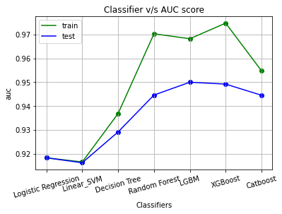
- Observations:
The performance of each model was recorded and plotted:
● The highest auc was achieved by LGBM with a score=95.00.
● Other ensemble models like random forest and XGBoost was also performing well.
● Linear models like logistic regression and linear SVM have achieved the minimum auc, ~0.917 & 0.914.
● All these model has achieved an AUC score > 0.91 while the maximum AUC achieved in the kaggle’s leaderboard was 0.88.
Feature Importance:
Computing Feature Importance is useful to know which features are more informative and contributing in prediction.By knowing the importance , we can reduce the no.of features by discarding less important features.
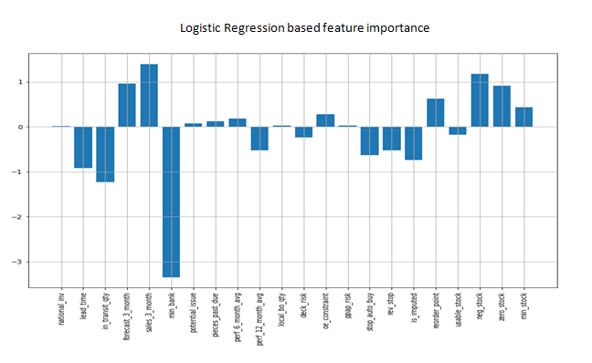
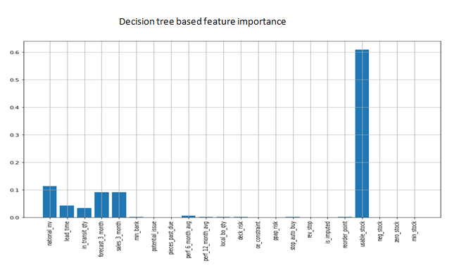
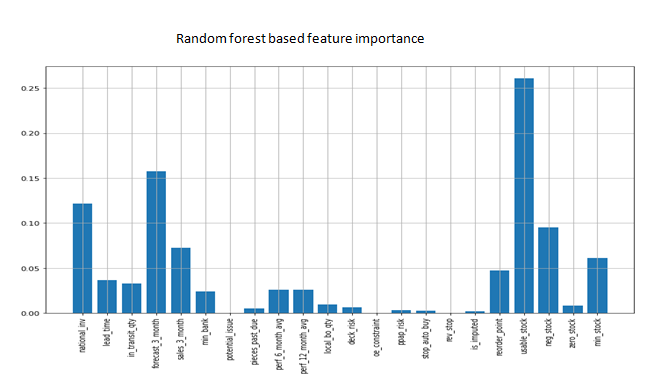
The Libraries has implemented built-in feature importance computation along with the algorithm implementations. In this case study, Logistic Regression based,decision tree based and Random Forest based feature importance where computed and plotted:
On analyzing the above plots, ‘usable_stock’ has showed high feature importance in the tree based models. ‘national_invariance’, forecast feature and ‘neg_stock’ were also having good feature importance. In tree based models, these important features are used for optimal splits of the nodes. Note that, ‘usable_stock’ and ‘neg_stock’ were the engineered features here.
In Logistic regression, feature importance is calculated as the weight associated with each feature. ‘min_bank’ has got highest negative weight, which means it the most important feature in predicting negative class. Other important features were ‘lead_time’, ‘in_transit_qty’, ‘forecast_3_months’, ‘neg_stock’ etc.
The least important features founded out were ‘potential_issue’, ‘local_bo_qty’, ‘oe_constraint’, ‘ppap_risk’, ‘rev_stop’ and ‘is_imputed’. These features were removed and the no.of features as reduced to 16,including engineered features before building the final model.
Final Model: Stacking Classifier
To enhance the performance of the individual models, a custom ensemble model was trained on the dataset by stacking the above mentioned individual models and the results were observed. Hyper-parameter tuning was employed to determine the best parameters for these models.
Performance:
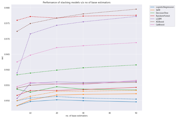
The no. of base estimators and the final stacking model was also determined by tuning. The Performance of different stacking models with different no. of base estimators:
The best performance was achieved with no.of models in the range 10–20 and LGBM as the stacking classifier with an auc of 95.50 . On further experimenting, 15 is chosen as the no. of base learners and LGBM as the stacking classifier which has improved the AUC to 96.39. The base learners were chosen by iterating through a list of models till the no. becomes 15.
Decision Threshold:
The model above computes probability of a point to belong to a particular class and AUC is computed using these probability scores. Class of a particular point is determined based on whether the predicted probability lies above or below a certain point called decision threshold. By default, it is taken as 0.5.
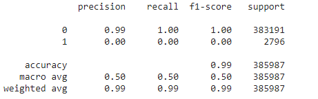
Even if the model achieved an AUC of 96.39 , the recall is 0 when taking 0.5 as decision threshold:
The Geometric Mean or G-Mean is a metric for imbalanced classification that, if optimized, will seek a balance between the sensitivity and the specificity.
G-means= sqrt(Sensitivity * Specificity) where,
Sensitivity = TruePositive / (TruePositive + FalseNegative)= tpr
Specificity = TrueNegative / (FalsePositive + TrueNegative)= 1-fpr
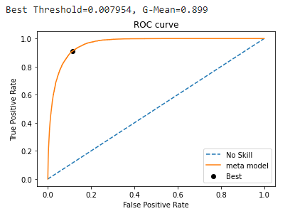
The ROC was plotted using a set of tpr and fpr at different decision thresholds. G-Mean for each threshold were calculated directly from these and the threshold which gives the maximum G-means was computed:
fpr,tpr,thresholds=roc_curve(y_test,test_pred)
gmeans=np.sqrt(tpr*(1-fpr))
ix=np.argmax(gmeans)
print('Best Threshold=%f, G-Mean=%.3f' % (thresholds[ix], gmeans[ix]))
# plot the roc curve for the model
plt.plot([0,1], [0,1], linestyle='--', label='No Skill')
plt.plot(fpr, tpr, marker='.', label='meta model')
plt.scatter(fpr[ix], tpr[ix], marker='o', color='black', label='Best')
which means, even if the model has placed positive points above negative points, none of them was identified as positive class. This why we should consider recall or f1 score instead of blindly relying on AUC only. Here the problem is with the default decision threshold. It should be lowered to get a reasonable recall. For this, an optimal threshold is found from ROC Curve by computing G-means.
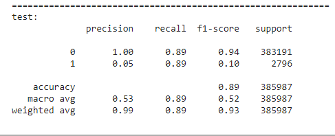
The decision threshold was calculated to be 0.0079. Any point with a predicted probability greater than this point will be classified as positive points. With this approach, the recall was computed to be:
The recall was improved to 0.89. Now the custom stacking model was built and deployed using streamlit. The App is running on material-backorder-prediction app.